Treatment effects often vary systematically with study-level characteristics — for example, the dose of an intervention or the year a study was conducted. metadid supports meta-regression by letting you include study-level covariates that modify the population treatment effect. This vignette walks through simulating data from a model with a single continuous covariate (dose) and fitting the meta-regression to recover both the intercept and slope.
Simulation
We simulate 40 studies where the true treatment effect depends
linearly on a covariate called dose. Higher doses produce a
more negative treatment effect:
library(metadid)
library(dplyr)
library(ggplot2)

dose <- seq(1, 4, length.out = 40)

sim <- simulate_meta_did(
  n_studies     = 40,
  n_control     = 100,
  n_treatment   = 100,
  true_effect   = -0.15,
  sigma_effect  = 0.03,
  true_trend    = -0.02,
  sigma_trend   = 0.01,
  baseline_mean = 0.45,
  baseline_sd   = 0.02,
  rho           = 0.5,
  seed          = 6427,
  covariates    = data.frame(dose = dose),
  beta_cov      = -0.04
)
The covariates argument takes a data frame with one row
per study, and beta_cov is a numeric vector of regression
coefficients (one per covariate column). Here, each unit increase in
dose shifts the raw treatment effect by -0.04.
True dose–effect relationship
Before fitting any model, we can inspect the true simulated treatment
effects. Each study has a known
stored in the true_params attribute. Dividing by the
study’s baseline level puts these on the normalised scale that the model
will estimate:
true_params <- attr(sim, "true_params")

params_with_dose <- true_params |>
  mutate(
    num = as.integer(gsub("study_", "", study_id)),
    dose = dose[num],
    normalised_effect = theta / baseline
  )

ggplot(params_with_dose, aes(x = dose, y = normalised_effect)) +
  geom_point() +
  geom_smooth(method = "lm", se = FALSE, linetype = "dashed") +
  labs(x = "Dose", y = "Normalised treatment effect") +
  theme_minimal()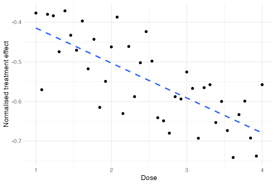
Higher doses produce more negative treatment effects, as specified by
beta_cov = -0.04. The scatter around the trend reflects
sigma_effect, the between-study heterogeneity that remains
after accounting for dose.
Understanding the true parameter values
Because meta_did() normalises outcomes by the baseline
mean (by default), the parameters the model estimates are on the
normalised scale. With a baseline mean of 0.45:
- True normalised slope:
- True normalised intercept at mean dose:
When center_covariates = TRUE (the default),
treatment_effect_mean is the effect evaluated at the mean
covariate value, not at dose = 0.
Extracting summary data
We extract full DiD summary statistics from all 40 studies. The
covariate column (dose) is carried through
automatically:
did_data <- as_summary_did(sim)

# Verify dose is present
did_data |>
  mutate(num = as.integer(gsub("study_", "", study_id))) |>
  arrange(num) |>
  select(study_id, design, dose) |>
  head()
#> # A tibble: 6 × 3
#> study_id design dose
#> <chr> <chr> <dbl>
#> 1 study_1 did 1
#> 2 study_2 did 1.08
#> 3 study_3 did 1.15
#> 4 study_4 did 1.23
#> 5 study_5 did 1.31
#> 6 study_6 did 1.38Fitting the meta-regression
Pass a one-sided formula to covariates to include the
meta-regression term:
#> Bayesian meta-analysis (metadid)
#> Studies: DiD = 40 | RCT = 0 | Pre-Post = 0 | DiD (change only) = 0
#> Population treatment effect: -0.538  90% CI [-0.560, -0.516]
#> Covariate coefficients:
#>   dose: -0.081  90% CI [-0.105, -0.057]
#>   (covariates were mean-centered; treatment_effect_mean is the effect at covariate means)
Both the intercept (treatment effect at mean dose) and the slope are recovered, with the true normalised values (-0.556 and -0.089) falling within the 90% credible intervals.
Inspecting the posterior
We can look at the full summary, including study-level treatment effects:
te <- summary(fit)
te[te$parameter %in% c("treatment_effect_mean", "treatment_effect_sd",
                        "beta_cov[dose]"), ]
#> parameter mean sd lo hi
#> 1 treatment_effect_mean -0.538 0.014 -0.560 -0.516
#> 2 treatment_effect_sd 0.077 0.010 0.061 0.095
#> 3 beta_cov[dose] -0.081 0.015 -0.105 -0.057The residual between-study SD (treatment_effect_sd)
represents the heterogeneity remaining after accounting for dose.
Estimated dose–effect relationship
A useful diagnostic is to plot the observed study-level treatment effects against the covariate and overlay the estimated regression line with uncertainty:
# Compute naive normalised effect per study
naive_effects <- did_data |>
  mutate(
    norm = mean_pre_control,
    naive_effect = (mean_post_treatment - mean_pre_treatment) / norm -
                   (mean_post_control - mean_pre_control) / norm
  )

# Posterior draws for regression line
beta_draws <- as.numeric(
  fit$fit$draws("beta_cov", format = "draws_matrix")
)
intercept_draws <- as.numeric(
  fit$fit$draws("treatment_effect_mean", format = "draws_matrix")
)

# Covariates were centered; reconstruct on original dose scale
dose_center <- fit$cov_centers[["dose"]]
dose_grid <- seq(min(dose), max(dose), length.out = 100)

# Each draw gives a line: intercept + beta * (dose - center)
line_df <- expand.grid(
  dose = dose_grid,
  draw = seq_along(beta_draws)
) |>
  mutate(
    fitted = intercept_draws[draw] + beta_draws[draw] * (dose - dose_center)
  ) |>
  group_by(dose) |>
  summarise(
    median = median(fitted),
    lo     = quantile(fitted, 0.05),
    hi     = quantile(fitted, 0.95),
    .groups = "drop"
  )

# True regression line on the normalised scale
true_line_df <- data.frame(dose = range(dose)) |>
  mutate(true_effect = (-0.15 + -0.04 * dose) / 0.45)

ggplot() +
  geom_ribbon(data = line_df, aes(x = dose, ymin = lo, ymax = hi),
              alpha = 0.2) +
  geom_line(data = line_df, aes(x = dose, y = median)) +
  geom_line(data = true_line_df, aes(x = dose, y = true_effect),
            linetype = "dashed", linewidth = 0.8) +
  geom_point(data = naive_effects, aes(x = dose, y = naive_effect),
             alpha = 0.6) +
  labs(x = "Dose", y = "Normalised treatment effect") +
  theme_minimal()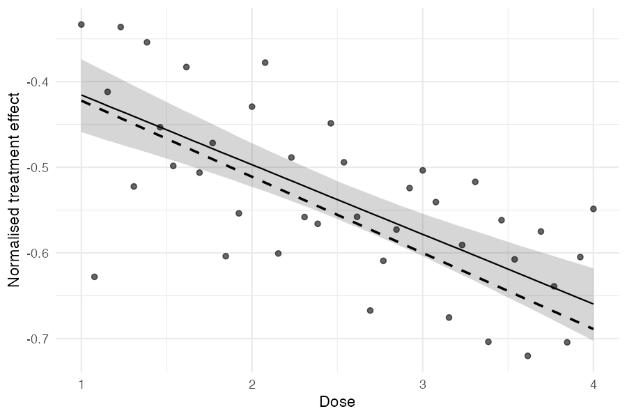
The points are naive study-level estimates, the solid line is the posterior median regression with a 90% credible band, and the dashed line is the true data-generating relationship.
Posterior predictive checks
The standard posterior predictive checks work with covariate models. The model-implied predictive distribution for each study accounts for its dose level:
pp_check_cdf(fit, type = "summary")Mixed designs with covariates
Covariates work with mixed-design meta-analyses too. For example, if some studies are RCTs and others are DiD, just ensure the covariate column is present in all rows of the combined summary data:
study_ids <- unique(sim$study_id)
true_params <- attr(sim, "true_params")

sim_did <- sim |> filter(study_id %in% study_ids[1:20])
sim_rct <- sim |> filter(study_id %in% study_ids[21:40])

attr(sim_did, "true_params") <- true_params |> filter(study_id %in% study_ids[1:20])
attr(sim_rct, "true_params") <- true_params |> filter(study_id %in% study_ids[21:40])

mixed_data <- bind_rows(
  as_summary_did(sim_did),
  as_summary_rct(sim_rct)
)

fit_mixed <- meta_did(
  summary_data = mixed_data,
  covariates   = ~ dose,
  seed         = 8153
)

print(fit_mixed)
#> Bayesian meta-analysis (metadid)
#> Studies: DiD = 20 | RCT = 20 | Pre-Post = 0 | DiD (change only) = 0
#> Population treatment effect: -0.544 90% CI [-0.567, -0.522]
#> Covariate coefficients:
#> dose: -0.086 90% CI [-0.111, -0.060]
#> (covariates were mean-centered; treatment_effect_mean is the effect at covariate means)The credible intervals are somewhat wider with mixed designs, but both the intercept and slope are still recovered.