Fitting real COVID-19 case data

library(epidp)
library(ggplot2)
library(dplyr)
#> 
#> Attaching package: 'dplyr'
#> The following objects are masked from 'package:stats':
#> 
#>     filter, lag
#> The following objects are masked from 'package:base':
#> 
#>     intersect, setdiff, setequal, union
library(magrittr)
library(purrr)
#> 
#> Attaching package: 'purrr'
#> The following object is masked from 'package:magrittr':
#> 
#>     set_names
library(tidyr)
#> 
#> Attaching package: 'tidyr'
#> The following object is masked from 'package:magrittr':
#> 
#>     extract

Estimating $R_t$ for Bogota using only the case data

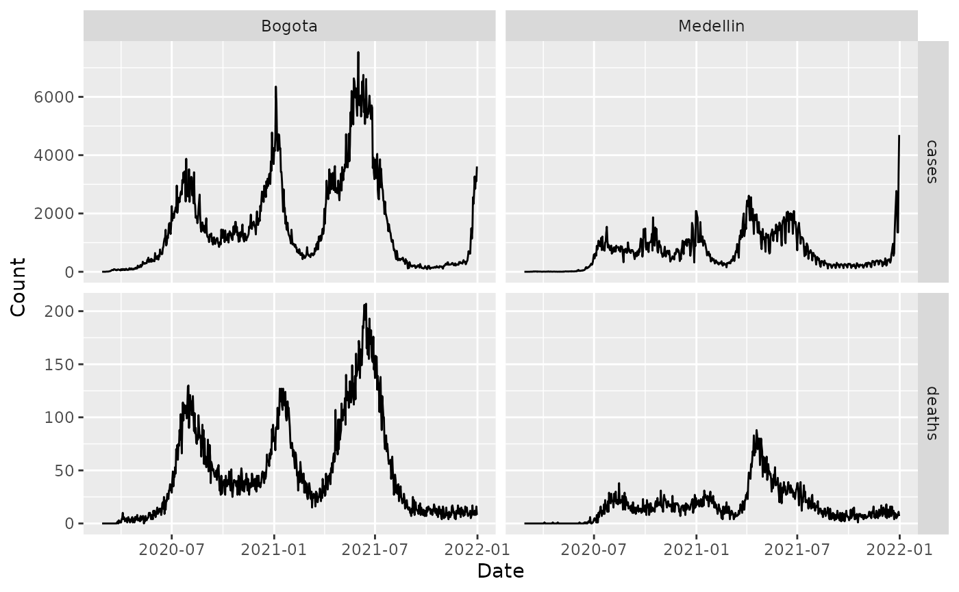
We first load the COVID-19 data for Colombia and graph it.

# load data
data("covid_colombia_cases_deaths_mobility")

# plot
covid_colombia_cases_deaths_mobility %>%
  pivot_longer(c(cases, deaths)) %>%
  ggplot(aes(x = date, y = value)) +
  geom_line() +
  facet_grid(vars(name), vars(city),
    scales = "free"
  ) +
  xlab("Date") +
  ylab("Count")

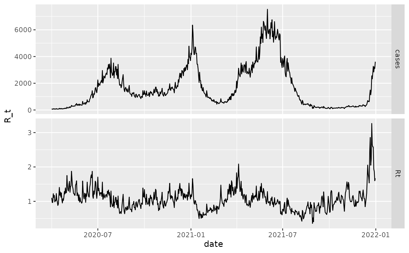
We first estimate $R_t$ for Bogota using only the case data using optimisation to give us a quick set of estimates.

df_bogota <- covid_colombia_cases_deaths_mobility %>%
  filter(city == "Bogota")

# generate serial interval for COVID-19 based on reasonable mean, sd
mean_si <- 6.5
sd_si <- 4.03
w <- generate_vector_serial(nrow(df_bogota), mean_si, sd_si)

# fit using optimisation
fit <- fit_epifilter(
  N = nrow(df_bogota),
  C = df_bogota$cases,
  w = w,
  is_sampling = FALSE,
  as_vector = FALSE
)

# plot
R <- fit$par$R
df_bogota %>%
  mutate(Rt = R) %>%
  select(date, Rt, cases) %>%
  filter(date >= as.Date("2020-04-01")) %>%
  pivot_longer(-date) %>%
  ggplot(aes(x = date, y = value)) +
  geom_line() +
  scale_color_brewer("R_t", palette = "Dark2") +
  ylab("R_t") +
  facet_grid(vars(name), scales = "free")

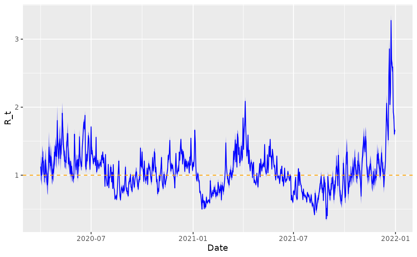
We now fit using a fully Bayesian framework which outputs uncertainty.

fit <- fit_epifilter(
  N = nrow(df_bogota),
  C = df_bogota$cases,
  w = w,
  is_sampling = TRUE,
  iter = 50,
  chains = 1 # as CRAN does not allow multiple cores
)
#> 
#> SAMPLING FOR MODEL 'epifilter' NOW (CHAIN 1).
#> Chain 1: 
#> Chain 1: Gradient evaluation took 0.014592 seconds
#> Chain 1: 1000 transitions using 10 leapfrog steps per transition would take 145.92 seconds.
#> Chain 1: Adjust your expectations accordingly!
#> Chain 1: 
#> Chain 1: 
#> Chain 1: WARNING: There aren't enough warmup iterations to fit the
#> Chain 1:          three stages of adaptation as currently configured.
#> Chain 1:          Reducing each adaptation stage to 15%/75%/10% of
#> Chain 1:          the given number of warmup iterations:
#> Chain 1:            init_buffer = 3
#> Chain 1:            adapt_window = 20
#> Chain 1:            term_buffer = 2
#> Chain 1: 
#> Chain 1: Iteration:  1 / 50 [  2%]  (Warmup)
#> Chain 1: Iteration:  5 / 50 [ 10%]  (Warmup)
#> Chain 1: Iteration: 10 / 50 [ 20%]  (Warmup)
#> Chain 1: Iteration: 15 / 50 [ 30%]  (Warmup)
#> Chain 1: Iteration: 20 / 50 [ 40%]  (Warmup)
#> Chain 1: Iteration: 25 / 50 [ 50%]  (Warmup)
#> Chain 1: Iteration: 26 / 50 [ 52%]  (Sampling)
#> Chain 1: Iteration: 30 / 50 [ 60%]  (Sampling)
#> Chain 1: Iteration: 35 / 50 [ 70%]  (Sampling)
#> Chain 1: Iteration: 40 / 50 [ 80%]  (Sampling)
#> Chain 1: Iteration: 45 / 50 [ 90%]  (Sampling)
#> Chain 1: Iteration: 50 / 50 [100%]  (Sampling)
#> Chain 1: 
#> Chain 1:  Elapsed Time: 15.566 seconds (Warm-up)
#> Chain 1:                21.413 seconds (Sampling)
#> Chain 1:                36.979 seconds (Total)
#> Chain 1:
#> Warning in validityMethod(object): The following variables have undefined
#> values: log_likelihood[1]. Many subsequent functions will not work correctly.
#> Warning: The largest R-hat is NA, indicating chains have not mixed.
#> Running the chains for more iterations may help. See
#> https://mc-stan.org/misc/warnings.html#r-hat
#> Warning: Bulk Effective Samples Size (ESS) is too low, indicating posterior means and medians may be unreliable.
#> Running the chains for more iterations may help. See
#> https://mc-stan.org/misc/warnings.html#bulk-ess
#> Warning: Tail Effective Samples Size (ESS) is too low, indicating posterior variances and tail quantiles may be unreliable.
#> Running the chains for more iterations may help. See
#> https://mc-stan.org/misc/warnings.html#tail-ess

# extract posterior quantiles
R_draws <- rstan::extract(fit, "R")[[1]]
lower <- apply(R_draws, 2, function(x) quantile(x, 0.025))
middle <- apply(R_draws, 2, function(x) quantile(x, 0.5))
upper <- apply(R_draws, 2, function(x) quantile(x, 0.975))

# plot
df_bogota %>%
  mutate(
    lower = lower,
    middle = middle,
    upper = upper
  ) %>%
  select(date, lower, middle, upper) %>%
  filter(date >= as.Date("2020-04-01")) %>%
  ggplot(aes(x = date)) +
  geom_ribbon(aes(ymin = lower, ymax = upper), fill = "blue", alpha = 0.6) +
  geom_line(aes(y = middle), colour = "blue") +
  geom_hline(yintercept = 1, linetype = 2, colour = "orange") +
  xlab("Date") +
  ylab("R_t")

Probing the drivers of $R_t$ using mobility data

We assume a relationship between workplace mobility $m_t$ and $R_t$ of the form:

$\log(R_t) = \alpha + \beta m_t + \epsilon_t,$

where $\epsilon_t$ represents the components of $R_t$ unrelated to workplace mobility.

We now fit this model using epidp.

X <- tibble(
  cons = rep(1, nrow(df_bogota)),
  m = df_bogota$workplaces
) %>%
  mutate(
    m = scale(m)[, 1]
  ) %>%
  as.matrix()

fit <- fit_epifilter_covariates(
  N = nrow(df_bogota),
  C = df_bogota$cases,
  w = w,
  X = X,
  is_sampling = TRUE,
  iter = 50, # probably too few iterations
  chains = 1 # as CRAN does not allow multiple cores; should run with more cores
)
#> 
#> SAMPLING FOR MODEL 'epifilter_covariates' NOW (CHAIN 1).
#> Chain 1: 
#> Chain 1: Gradient evaluation took 0.01527 seconds
#> Chain 1: 1000 transitions using 10 leapfrog steps per transition would take 152.7 seconds.
#> Chain 1: Adjust your expectations accordingly!
#> Chain 1: 
#> Chain 1: 
#> Chain 1: WARNING: There aren't enough warmup iterations to fit the
#> Chain 1:          three stages of adaptation as currently configured.
#> Chain 1:          Reducing each adaptation stage to 15%/75%/10% of
#> Chain 1:          the given number of warmup iterations:
#> Chain 1:            init_buffer = 3
#> Chain 1:            adapt_window = 20
#> Chain 1:            term_buffer = 2
#> Chain 1: 
#> Chain 1: Iteration:  1 / 50 [  2%]  (Warmup)
#> Chain 1: Iteration:  5 / 50 [ 10%]  (Warmup)
#> Chain 1: Iteration: 10 / 50 [ 20%]  (Warmup)
#> Chain 1: Iteration: 15 / 50 [ 30%]  (Warmup)
#> Chain 1: Iteration: 20 / 50 [ 40%]  (Warmup)
#> Chain 1: Iteration: 25 / 50 [ 50%]  (Warmup)
#> Chain 1: Iteration: 26 / 50 [ 52%]  (Sampling)
#> Chain 1: Iteration: 30 / 50 [ 60%]  (Sampling)
#> Chain 1: Iteration: 35 / 50 [ 70%]  (Sampling)
#> Chain 1: Iteration: 40 / 50 [ 80%]  (Sampling)
#> Chain 1: Iteration: 45 / 50 [ 90%]  (Sampling)
#> Chain 1: Iteration: 50 / 50 [100%]  (Sampling)
#> Chain 1: 
#> Chain 1:  Elapsed Time: 6.076 seconds (Warm-up)
#> Chain 1:                58.014 seconds (Sampling)
#> Chain 1:                64.09 seconds (Total)
#> Chain 1:
#> Warning in validityMethod(object): The following variables have undefined
#> values: log_likelihood[1]. Many subsequent functions will not work correctly.
#> Warning: There were 1 chains where the estimated Bayesian Fraction of Missing Information was low. See
#> https://mc-stan.org/misc/warnings.html#bfmi-low
#> Warning: Examine the pairs() plot to diagnose sampling problems
#> Warning: The largest R-hat is NA, indicating chains have not mixed.
#> Running the chains for more iterations may help. See
#> https://mc-stan.org/misc/warnings.html#r-hat
#> Warning: Bulk Effective Samples Size (ESS) is too low, indicating posterior means and medians may be unreliable.
#> Running the chains for more iterations may help. See
#> https://mc-stan.org/misc/warnings.html#bulk-ess
#> Warning: Tail Effective Samples Size (ESS) is too low, indicating posterior variances and tail quantiles may be unreliable.
#> Running the chains for more iterations may help. See
#> https://mc-stan.org/misc/warnings.html#tail-ess

print(fit, "beta[2]")
#> Inference for Stan model: epifilter_covariates.
#> 1 chains, each with iter=50; warmup=25; thin=1; 
#> post-warmup draws per chain=25, total post-warmup draws=25.
#> 
#>          mean se_mean   sd  2.5%   25%   50%   75% 97.5% n_eff Rhat
#> beta[2] -0.06    0.01 0.01 -0.08 -0.07 -0.05 -0.05 -0.04     4 1.47
#> 
#> Samples were drawn using NUTS(diag_e) at Thu Nov 14 19:26:15 2024.
#> For each parameter, n_eff is a crude measure of effective sample size,
#> and Rhat is the potential scale reduction factor on split chains (at 
#> convergence, Rhat=1).

This negative association probably is a result of individuals responding to the COVID-19 pandemic conditions or governmental policy.

Determining drivers of $R_t$ for Bogota using financial time series

data("bogota_financial_time_series")

Smooth the weekly time series

daily_dates <- seq(
  min(bogota_financial_time_series$date),
  max(bogota_financial_time_series$date), by = "day")

merchants <- unique(bogota_financial_time_series$merch_category)
for(i in seq_along(merchants)) {
  df_short <- bogota_financial_time_series %>% 
    filter(merch_category==merchants[i])
  spendamountusd_interpolated <- approx(
    df_short$date,
    df_short$spendamt, xout = daily_dates)$y
  countamountusd_interpolated <- approx(df_short$date, df_short$nb_transactions, xout = daily_dates)$y
  df_daily <- tibble(
      date=daily_dates,
      spendamountusd=spendamountusd_interpolated,
      countamountusd=countamountusd_interpolated
      ) %>% 
    mutate(merch_type=merchants[i])
  
  if(i == 1)
    big_df <- df_daily
  else
    big_df <- big_df %>% bind_rows(df_daily)
}

df_both <- big_df %>% 
  left_join(covid_colombia_cases_deaths_mobility) %>% 
  filter(city=="Bogota")
#> Joining with `by = join_by(date)`
#> Warning in left_join(., covid_colombia_cases_deaths_mobility): Detected an unexpected many-to-many relationship between `x` and `y`.
#> ℹ Row 423 of `x` matches multiple rows in `y`.
#> ℹ Row 1 of `y` matches multiple rows in `x`.
#> ℹ If a many-to-many relationship is expected, set `relationship =
#>   "many-to-many"` to silence this warning.

Here, we demonstrate how we can investigate whether the (smoothed) daily number of transactions in Bogota is associated with $R_$. We pick the “Grocery Stores/Supermarkets” category here because this is likely a particularly high contact shop.

df_supermarkets <- df_both %>% 
  filter(merch_type=="Grocery Stores/Supermarkets")

X <- tibble(
  cons = rep(1, nrow(df_bogota)),
  m = df_supermarkets$countamountusd
) %>%
  mutate(
    m = scale(m)[, 1]
  ) %>%
  as.matrix()

options(mc.cores=4)
fit <- fit_epifilter_covariates(
  N = nrow(df_supermarkets),
  C = df_supermarkets$cases,
  w = w,
  X = X,
  is_sampling = TRUE,
  iter = 200,
  chains = 4 
)
#> Warning in validityMethod(object): The following variables have undefined
#> values: log_likelihood[1]. Many subsequent functions will not work correctly.
#> Warning: There were 1 transitions after warmup that exceeded the maximum treedepth. Increase max_treedepth above 10. See
#> https://mc-stan.org/misc/warnings.html#maximum-treedepth-exceeded
#> Warning: Examine the pairs() plot to diagnose sampling problems
#> Warning: The largest R-hat is NA, indicating chains have not mixed.
#> Running the chains for more iterations may help. See
#> https://mc-stan.org/misc/warnings.html#r-hat
#> Warning: Bulk Effective Samples Size (ESS) is too low, indicating posterior means and medians may be unreliable.
#> Running the chains for more iterations may help. See
#> https://mc-stan.org/misc/warnings.html#bulk-ess
#> Warning: Tail Effective Samples Size (ESS) is too low, indicating posterior variances and tail quantiles may be unreliable.
#> Running the chains for more iterations may help. See
#> https://mc-stan.org/misc/warnings.html#tail-ess

print(fit, "beta[2]")

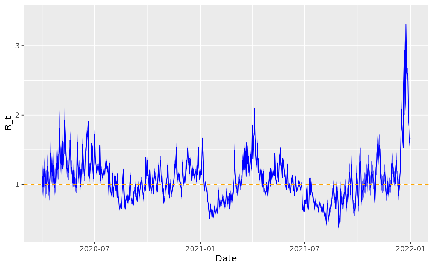
Plotting $R_t$ using these estimates.

# extract posterior quantiles
R_draws <- rstan::extract(fit, "R")[[1]]
lower <- apply(R_draws, 2, function(x) quantile(x, 0.025))
middle <- apply(R_draws, 2, function(x) quantile(x, 0.5))
upper <- apply(R_draws, 2, function(x) quantile(x, 0.975))

# plot
df_supermarkets %>%
  mutate(
    lower = lower,
    middle = middle,
    upper = upper
  ) %>%
  select(date, lower, middle, upper) %>%
  filter(date >= as.Date("2020-04-01")) %>%
  ggplot(aes(x = date)) +
  geom_ribbon(aes(ymin = lower, ymax = upper), fill = "blue", alpha = 0.6) +
  geom_line(aes(y = middle), colour = "blue") +
  geom_hline(yintercept = 1, linetype = 2, colour = "orange") +
  xlab("Date") +
  ylab("R_t")

Estimating RtR_t for Bogota using only the case data

Probing the drivers of RtR_t using mobility data

Determining drivers of RtR_t for Bogota using financial time series

Estimating $R_t$ for Bogota using only the case data

Probing the drivers of $R_t$ using mobility data

Determining drivers of $R_t$ for Bogota using financial time series